The Order of Operation is the single most important concept you need to understand during your journey to learn Tableau.
So what is the Order of Operation in the first place? Simply stated it is the sequence Tableau follows each time you create a new worksheet. I like to use the 10-step model viewed in 3 groups:
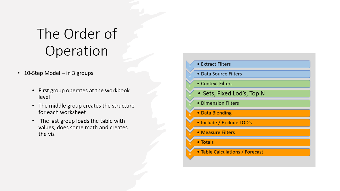
The first 2 steps operate at the workbook level and can improve the performance of the workbook. The remaining steps are executed with each new worksheet. Steps 3-5 create the structure for the data table for the sheet while the remaining 5 steps (6-10) load the table with data, perform calculations and create the viz.
Here we will look at how specific steps affect simple and more complex calculations.
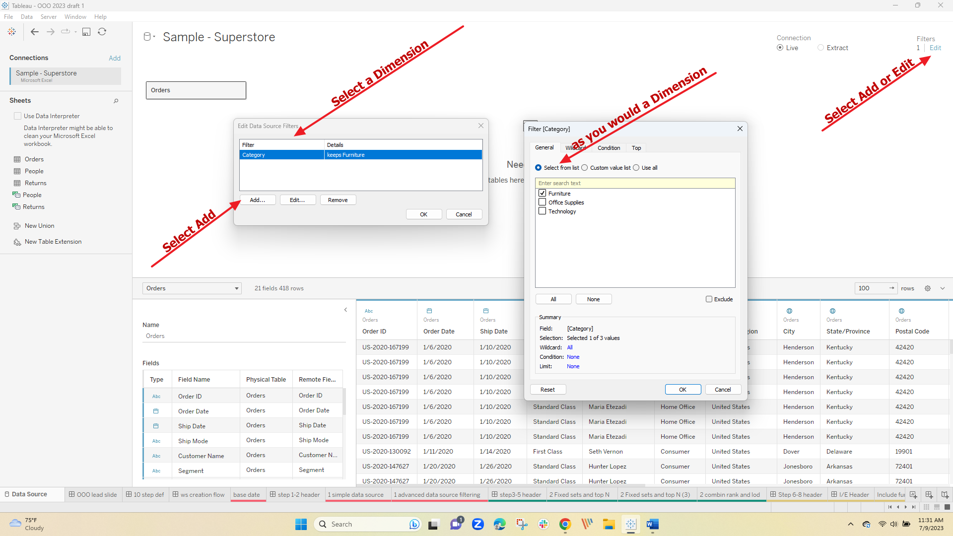
Steps 1-2 Data Source and Extract Filters
These filters reduce the workbook's data when files are uploaded into Tableau. Eliminating unneeded data will make to workbook perform better. They are very easy to use and applied on the Data Source tab. In their most basic form, it is similar to adding a dimension filter. From the data source tab select ADD and the dimension to filter and the values to keep. In this example keeping only furniture reduced the number of records from 10K to 2200 –
Now for the more advanced version using a conditional expression – conditions that can be determined at the time the data is loaded, it can be used to create a dynamic filter –
For this example I only want to include customers whose total sales are greater than 10K. Since the expression is calculated as the data is loaded the filter is applied dynamically each time the data is updated
The LOD is:
{ FIXED [Customer Name]: sum([Sales])>10000 }
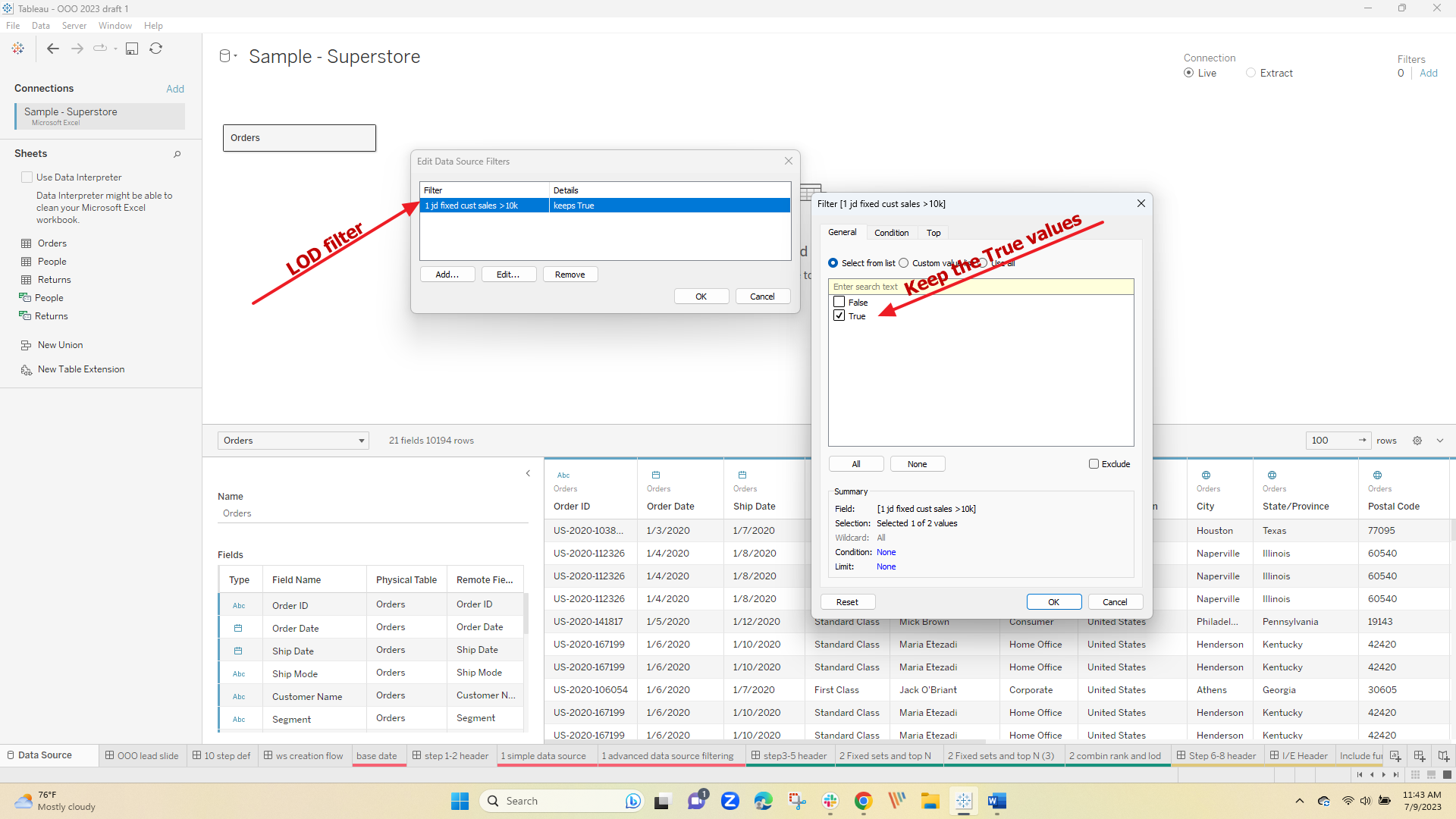
The LOD is selected from the dropdown and set to True – as a result the number of customers in the dataset is reduced from 800 to 21 that have sales greater than 10k with a total record count of 418.
Steps 3-5 Context Filters, Fixed LOD, Sets, Top N and Dimension Filters
For new and experienced users alike, when and how to apply Context filters causes most of their errors. If you get nothing else from this post just remember this – a dimension in Context is filtered before the Fixed LOD is calculated, Sets are created or the Top N is determined. Dimensions not in Context will be filtered after.
Ok not so hard – let's look at some basic examples:
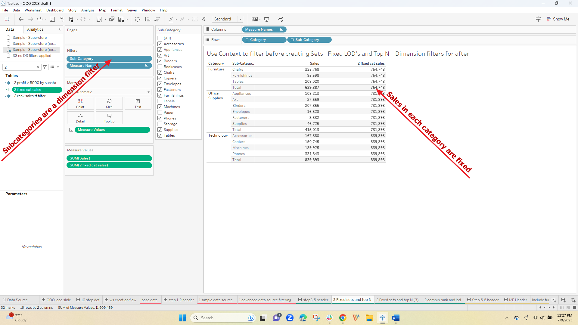
In this first example, the Sales at the Category and Year level are fixed with this:
{ FIXED [Category],year([Order Date]):sum([Sales])}
The total sales in each category are fixed – even when we apply a filter on the subcategory as a dimension filter (blue pill) the value remains unchanged (Ie the filter is applied to the subcategory after the LOD is calculated.
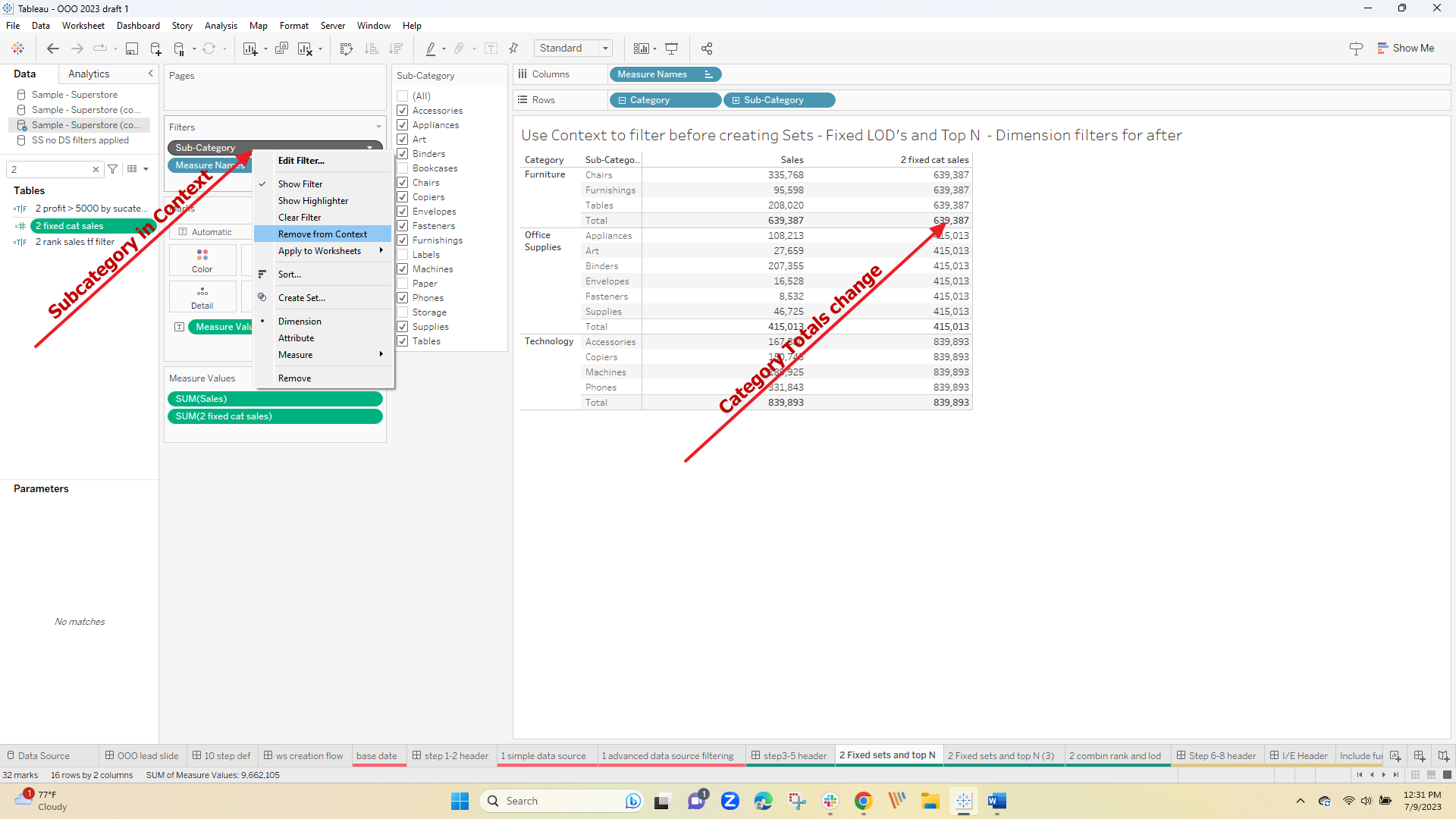
When Subcategory is placed in Context (Gray pill) the filter is applied before the LOD is calculated so the total for each category now reflects the filtering
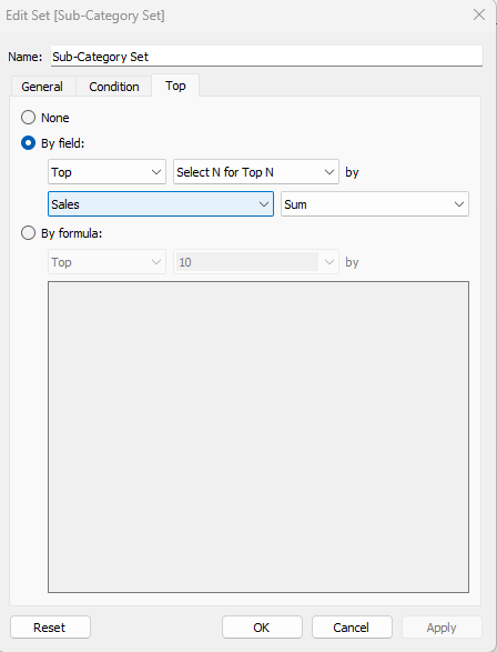
Something similar happens when we use Top N – I created a set on Subcategory using the Top N option
Applying a filter to a subcategory and the filter is a blue pill (dimension filter) the filter is applied after the Top N are determined only 2 subcategories are in the set
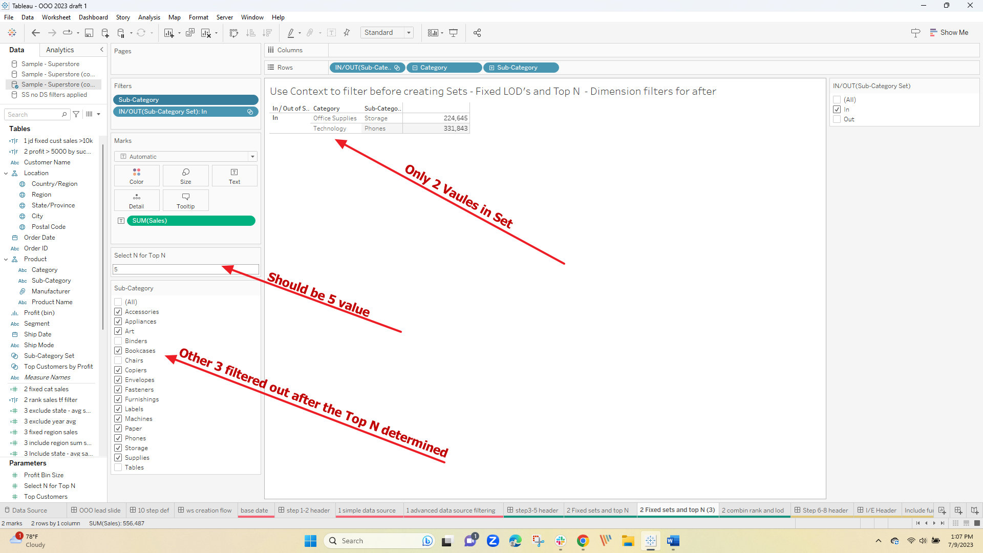
If I place the filter in Context – 5 subcategories are returned and they are the Top 5 of the remaining 14 after the 3 were filtered out
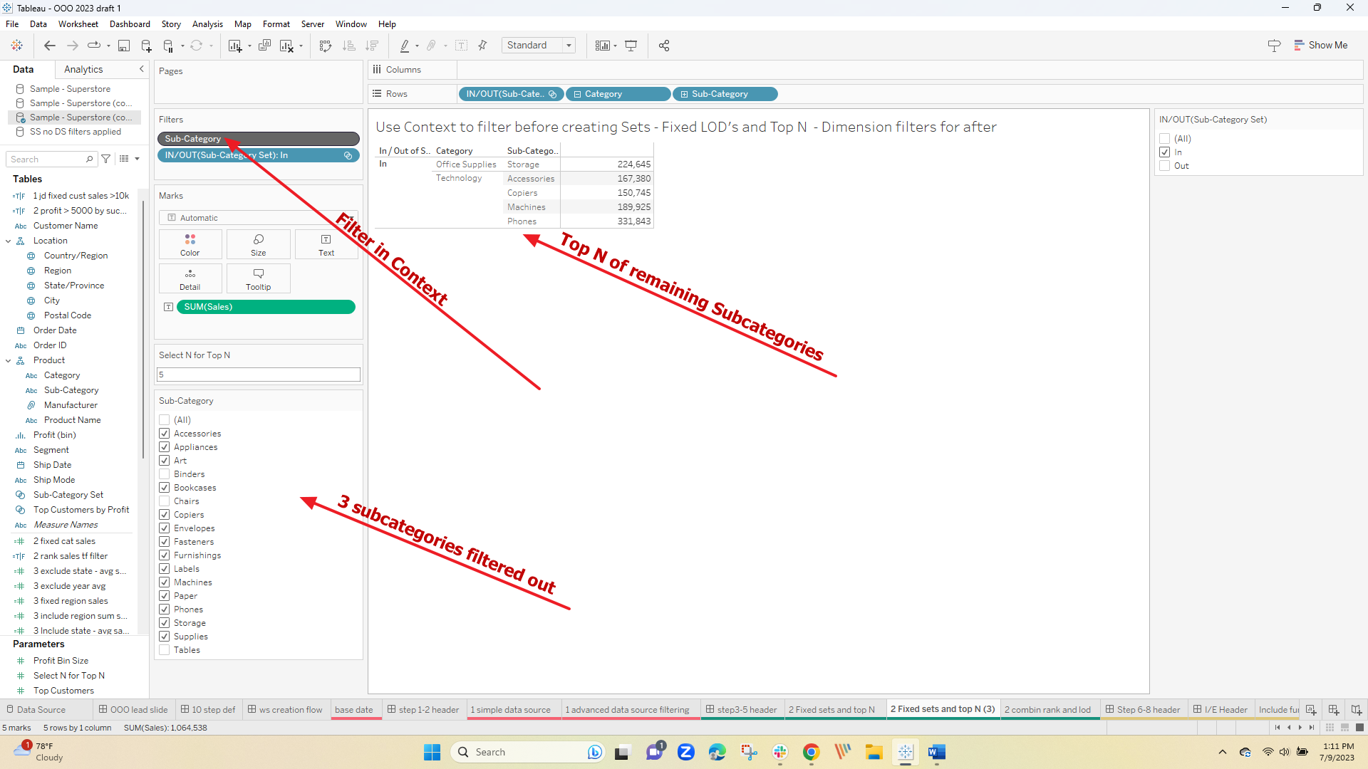
So the rule still applies – Dimensions in Context are applied before Fixed LODs, Set or Top N are applied and Dimensions filters applied NOT in context do not affect those values.
But what happens when you need to filter applied to a Fixed LOD and to a Top N? – That leads to the advanced case because Fixed LODs and Top N are both determined in the same step of the Order of Operations. – In the example, we try to apply a filter for this LOD
{ FIXED [Sub-Category]:sum([Profit])}>5000
And also take a Top N based on Sales but we can't get both filters to work properly together
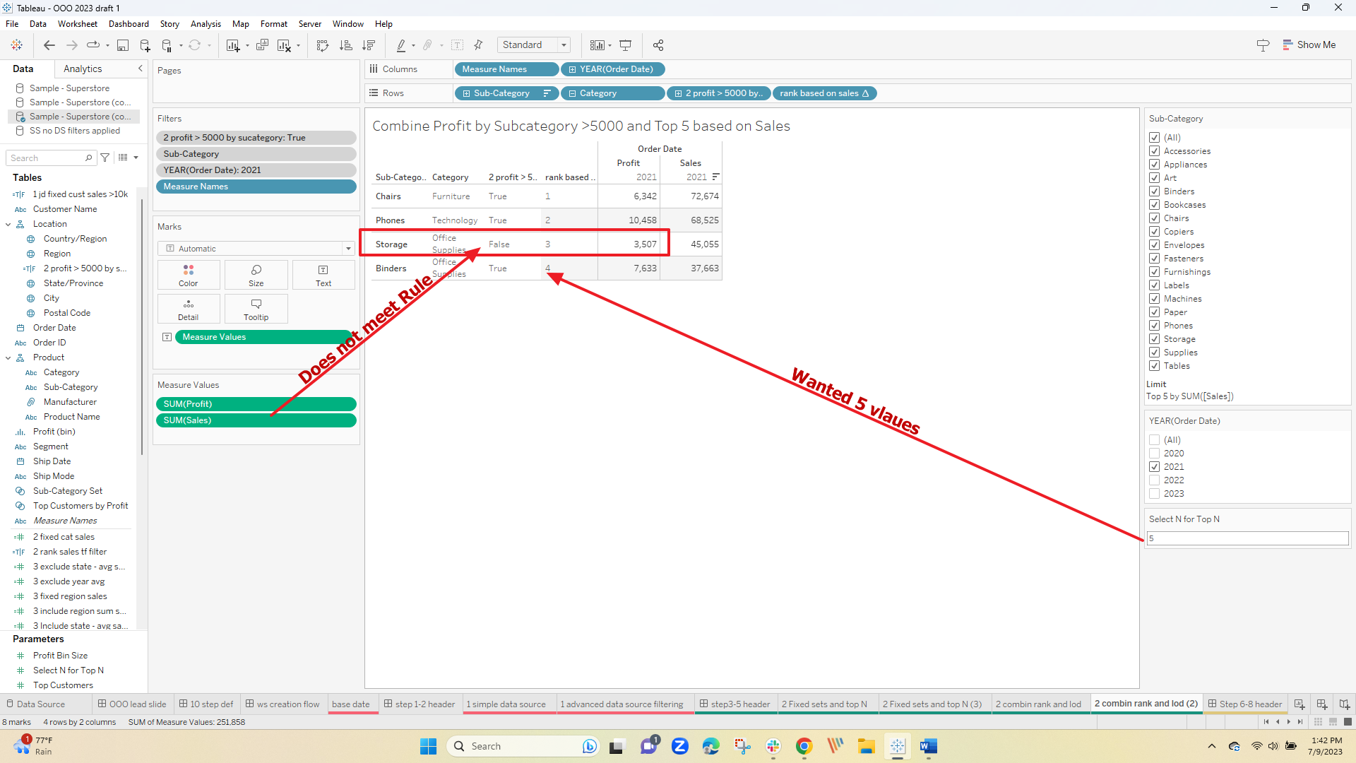
We have to go back to the Order of Operation and find an alternate way to find the top-performing subcategories that also meet the min profit goal. That can be accomplished by ranking the subcategories using a table calculation
RANK_UNIQUE(sum( { FIXED [Sub-Category]:sum([Sales])} ),'desc')
And then using a Boolean filter based on a rank less than a parameter value
[2 rank based on sales]<=[Select N for Top N]
Combined they now return this
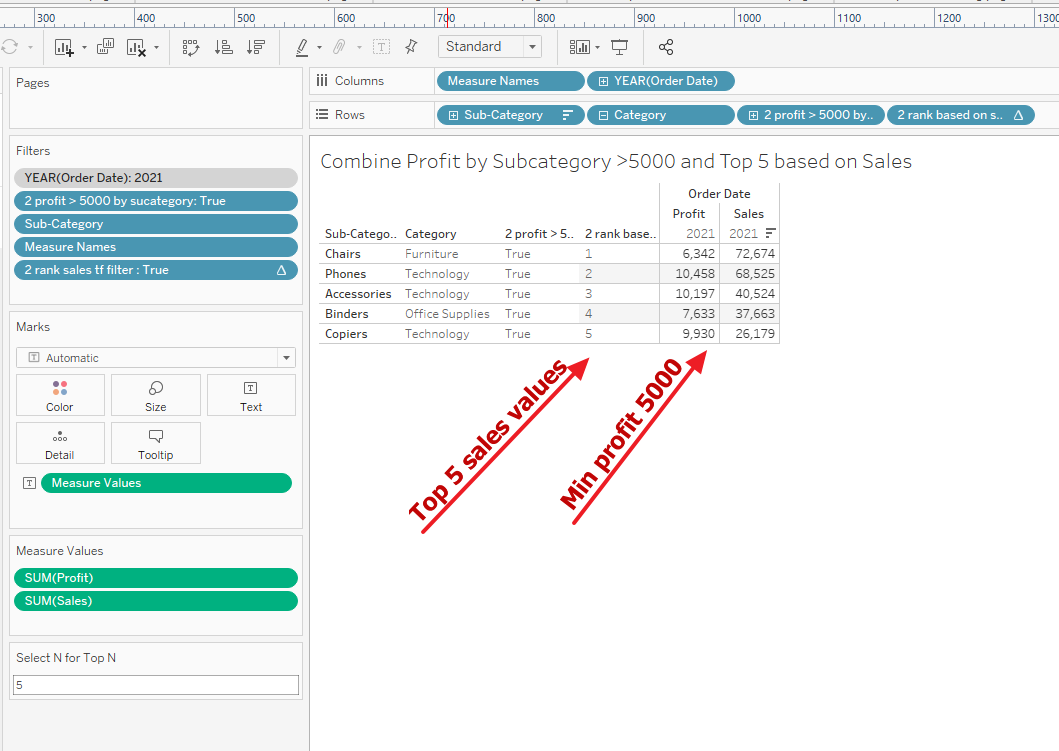
Steps 6-10 in the Order of Operation
The remaining steps fill the worksheet data table with data, perform some calculations and create the viz. Here we will only focus on steps that involve calculations.
Step 7 Include and Exclude LODs
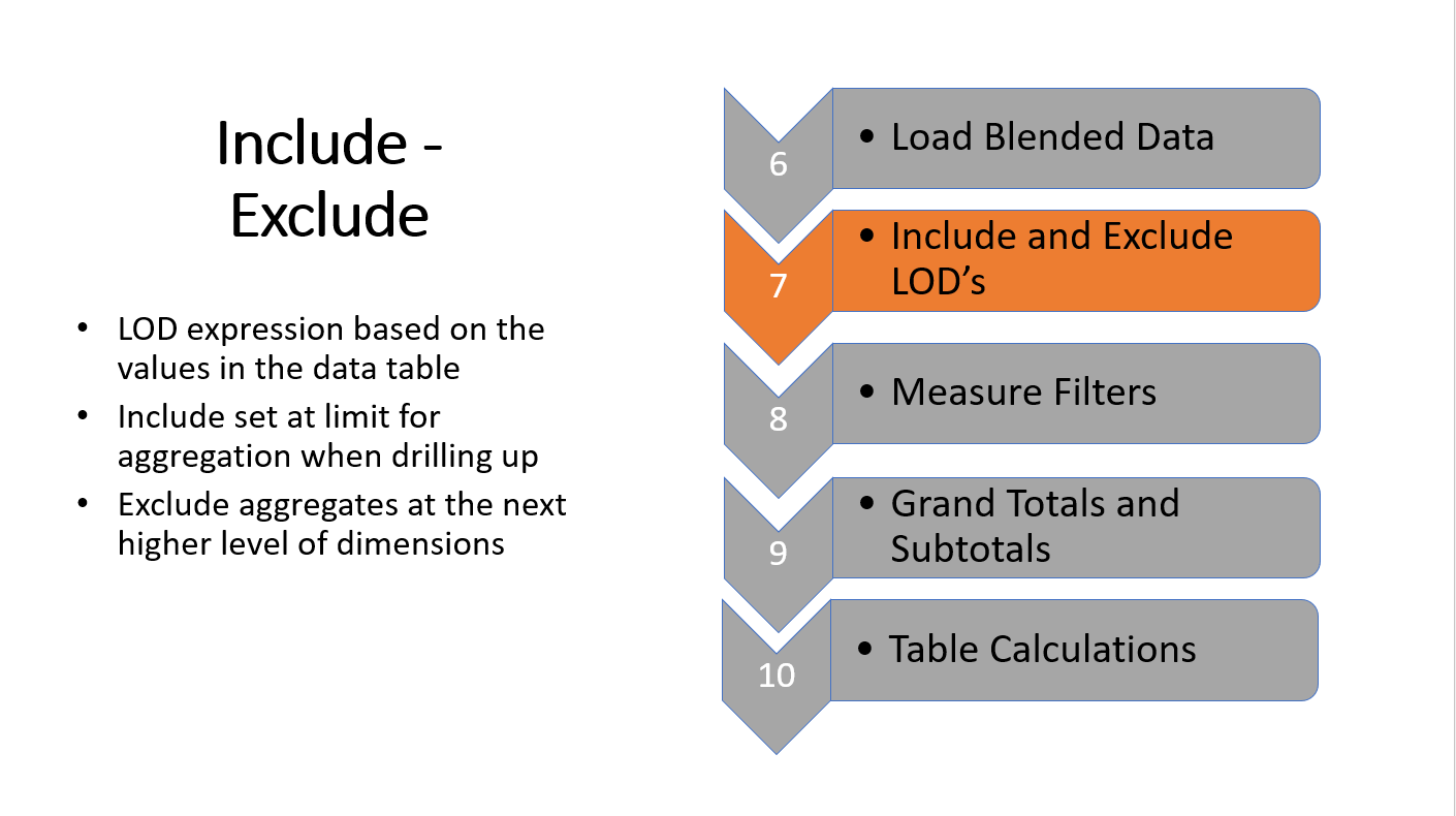
Include and exclude are LODs that operate on values in the data table. They are used in about 20% of use cases and often lead to confusion.
The Include statement can be used to set the upper limit for the aggregation in a LOD – it is easier to understand in this example:
{ INCLUDE [State/Province]:AVG([Sales])}
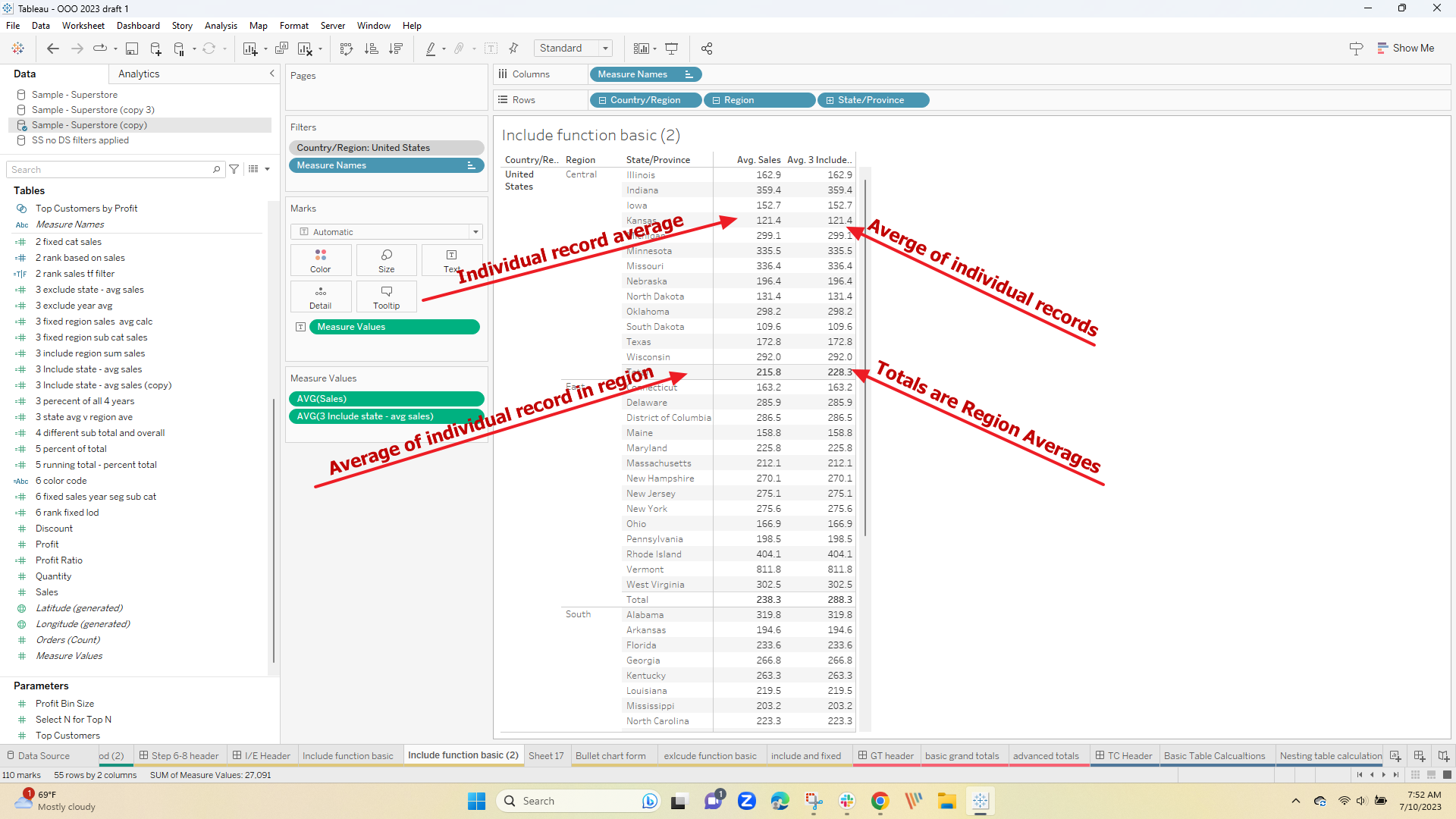
At the "Region" level and above, the statement calculates the average of the within each region and then aggregates that total
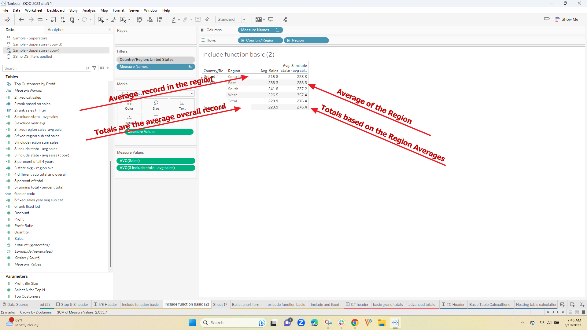
At lower levels in the viz include returns the same averages as those for the individual records – the automatic totals will reflect the regions averages
Exclude aggregates values at the next hirer level dimension in the viz – Again an example is easier to see using this:
{ EXCLUDE [State/Province]:AVG([Sales])}
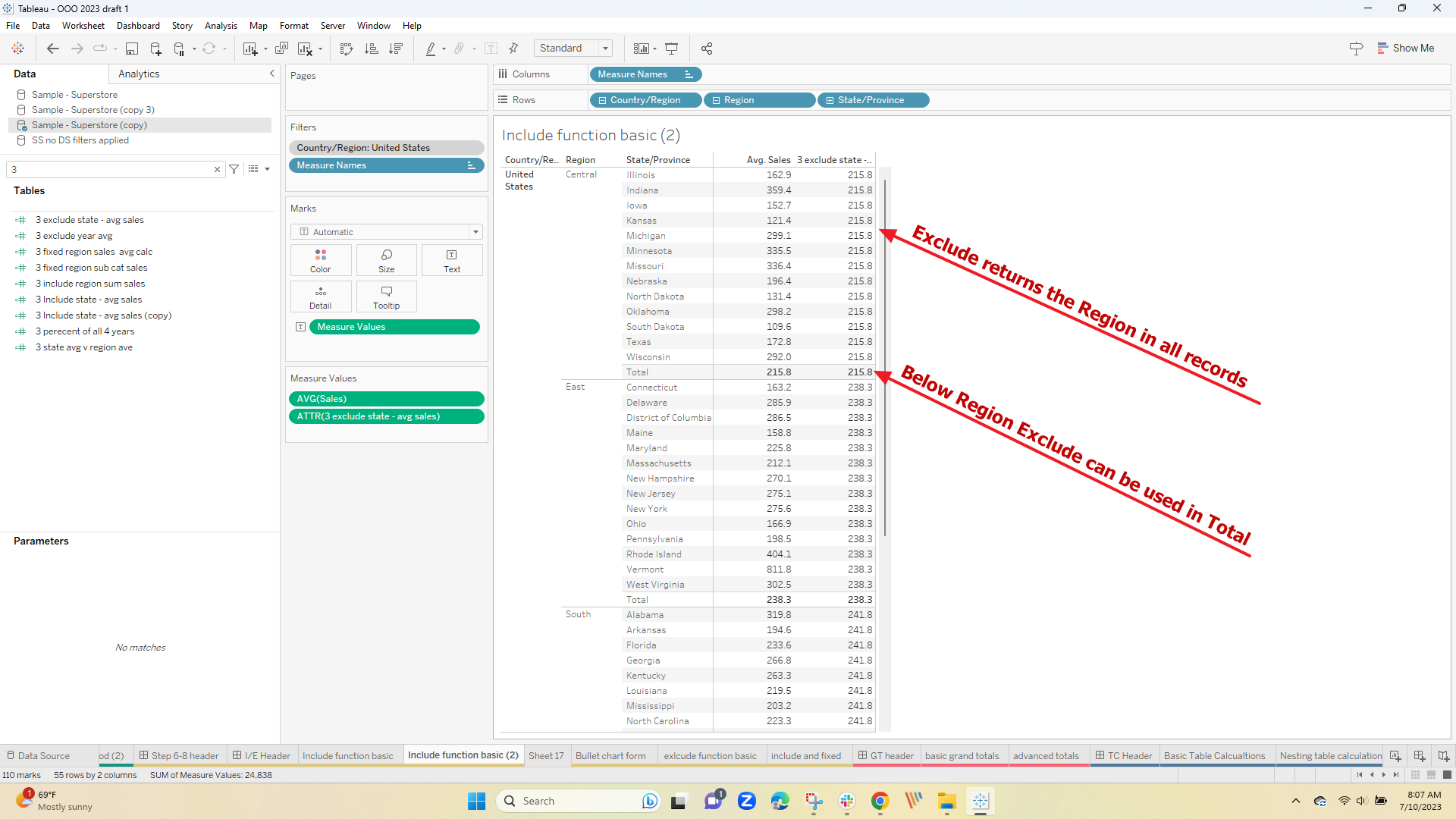
Excluding the State will return the Region averages at the region level in the viz but note it can not be used in Grand Totals
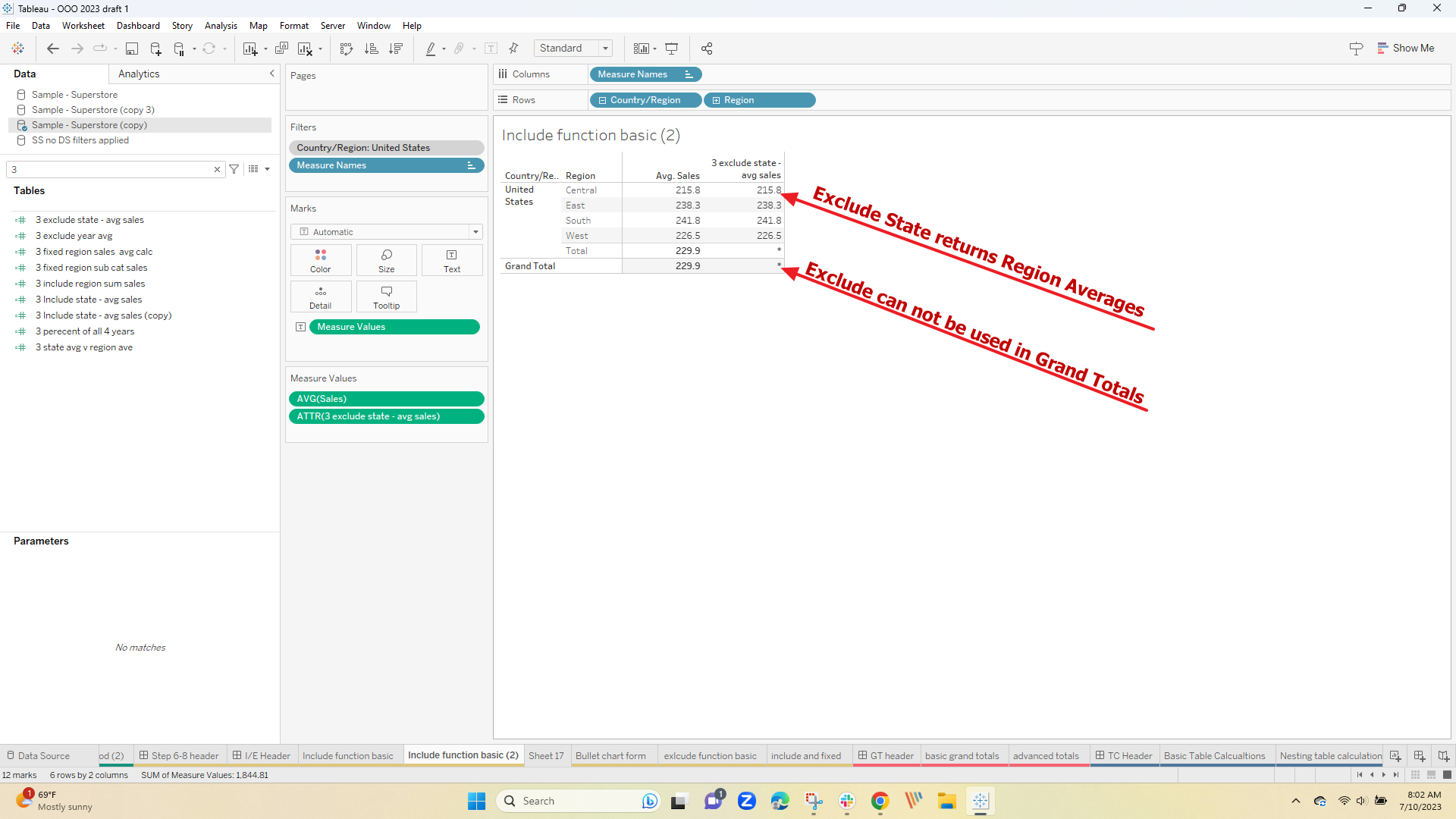
At levels below region Exclude returns the Region's total
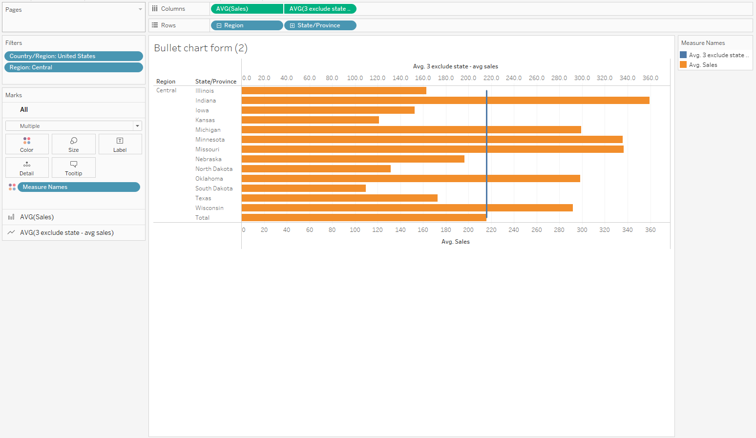
Hope that clears up how to use Include and Exclude – an interesting use case is to create a bullet chart
Grand Totals
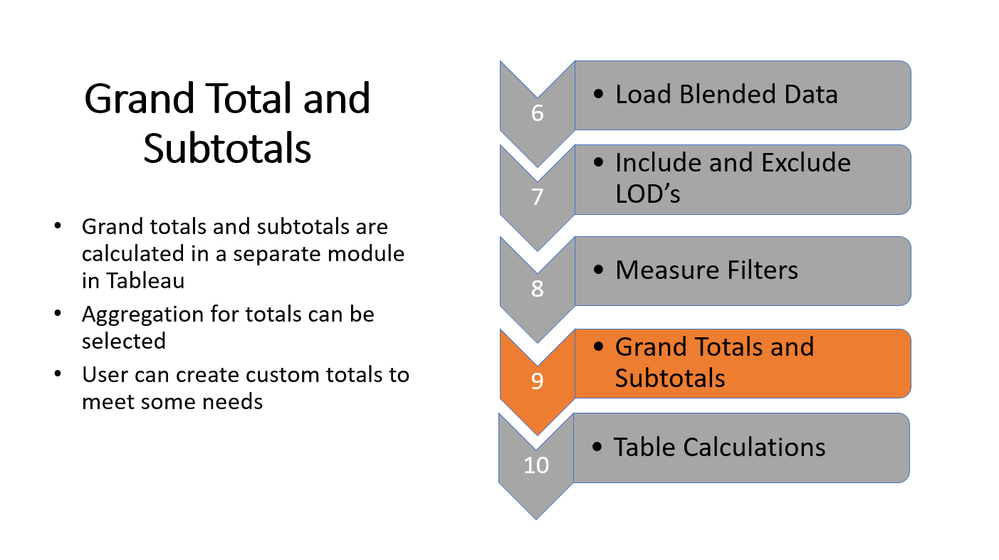
Basic Grand Totals and Subtotals are very easy to use – just remember that Tableau calculates the values in a separate module and based on the filtered data table for the worksheet – for a complete explanation see Totals and subtotals
You can simply drag and drop Grand Totals from the analytics tab
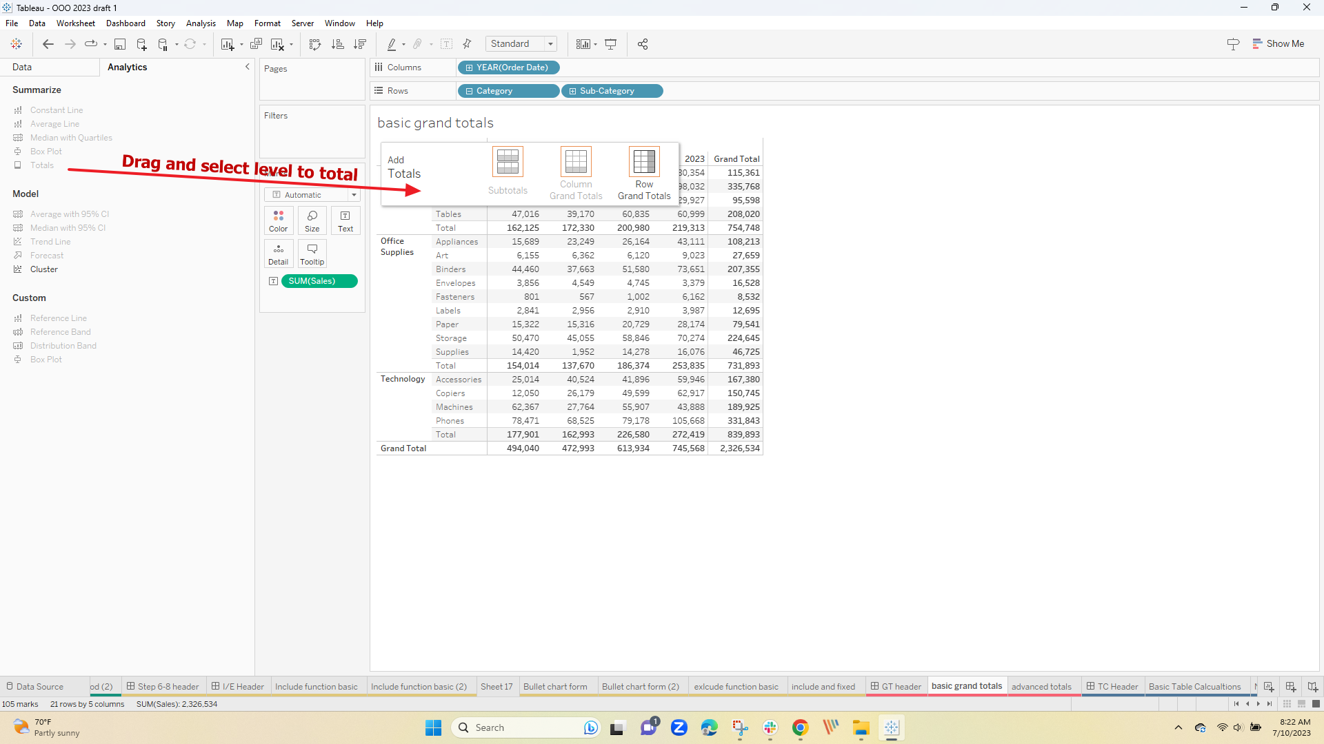
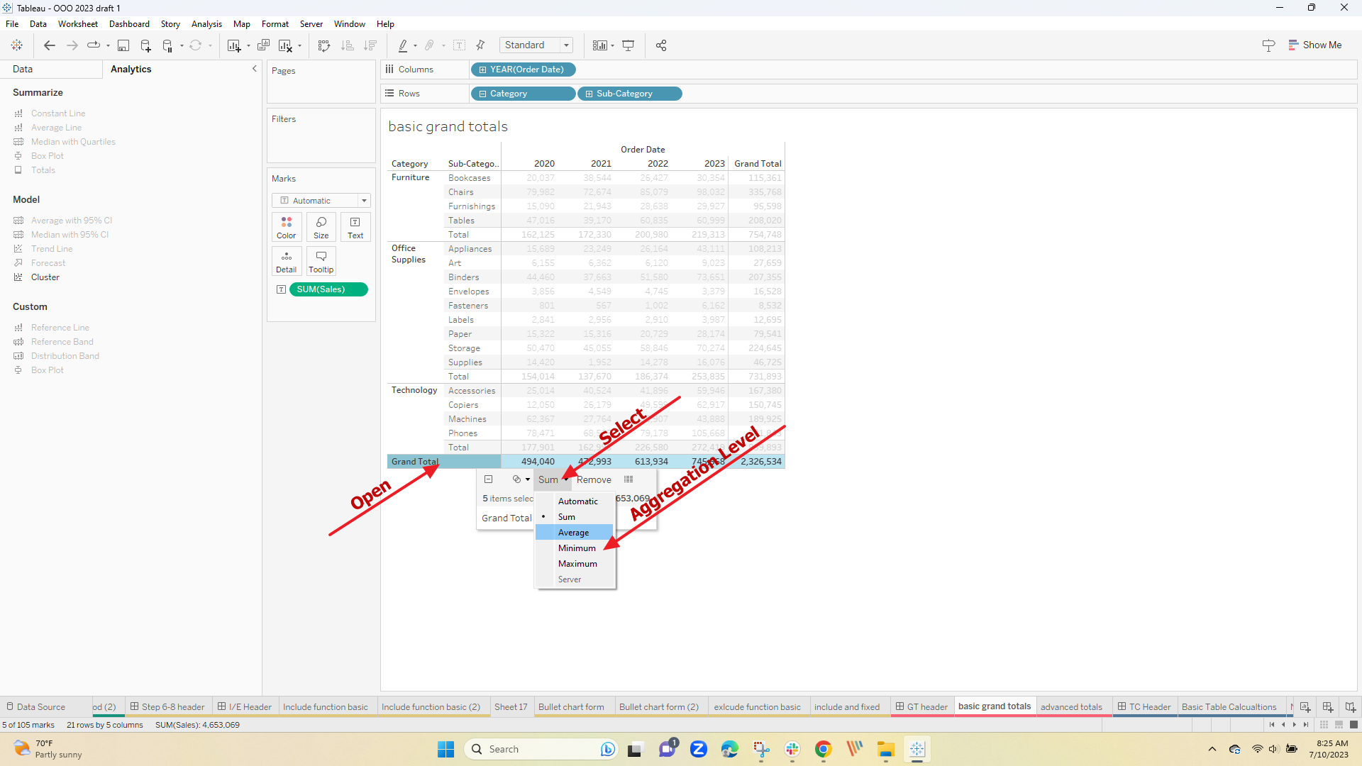
The default aggregation is Automatic (that is based on your custom calculation or sum()) but you can adjust that as needed
Sometimes the built-in aggregations don't result in what you expected – in most of those cases, you can use a custom expression to create totals. In this use case, the percent of total category is calculated for each subcategory at the row level but the category percent to overall total sales is presented at the subtotal levels
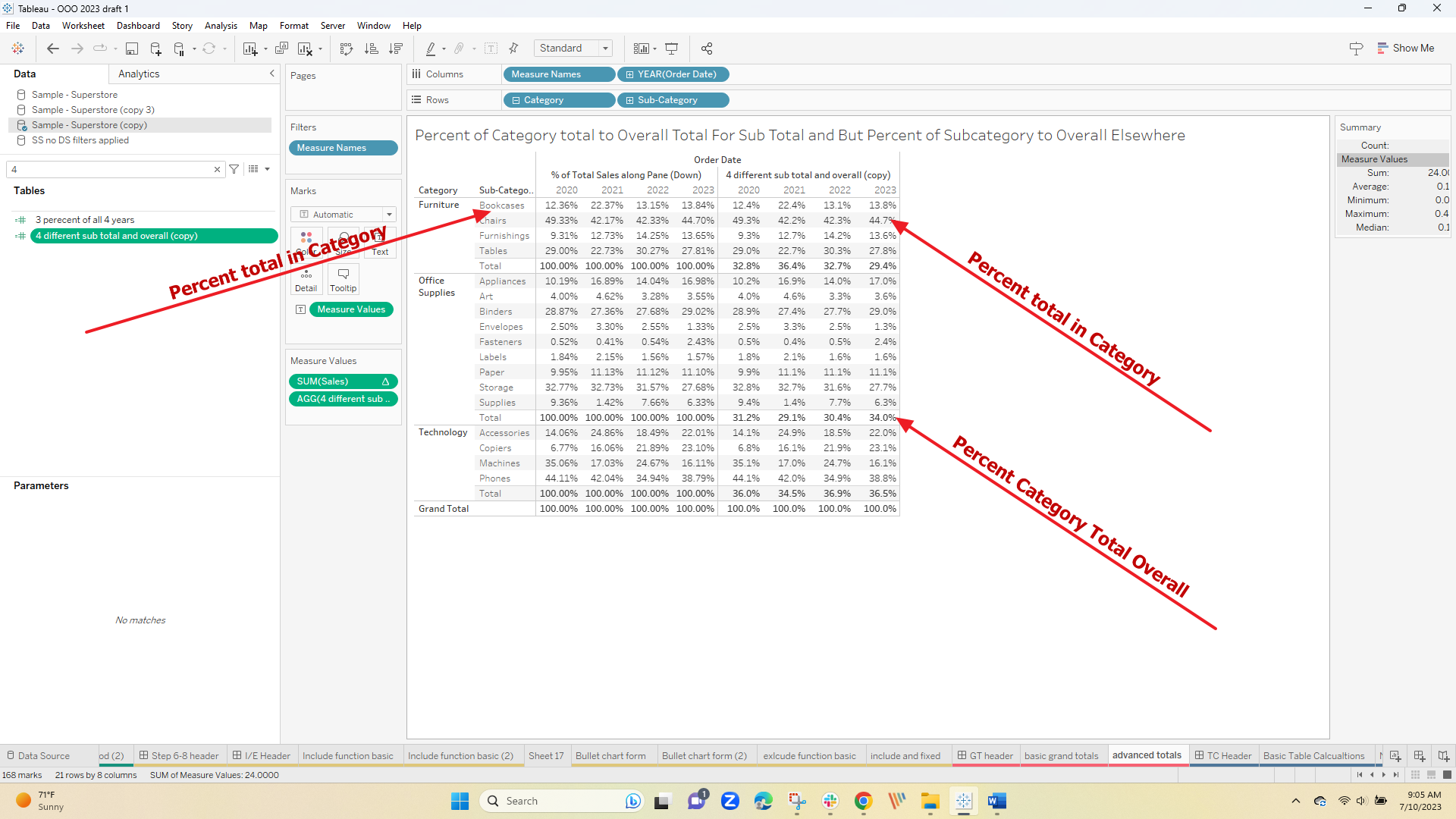
It is done with this formula
if max([Sub-Category])<>min([Sub-Category])
then Sum({ FIXED [Category],year([Order Date]):sum([Sales])})/
Sum({ FIXED year([Order Date]):sum([Sales])})
Else
Sum({ FIXED Year([Order Date]),[Sub-Category]:sum([Sales])})/
Sum({ FIXED Year([Order Date]),[Category]:sum([Sales])}) end
The formula takes advantage of the fact the subtotal and grand total "rows" are calculated in a separate module – the first condition is to test if the min subcategory is the same as the max (that is true for each of the line item row but not in the subtotal for the category – when that is found the "Then" clause is explicitly formula to apply in that row – the Else clause is just the formula use elsewhere.
The same approach can be used to sub-total multiple layers in a drill-down hierarchy – see Multi-layer custom totals
Table Calculations
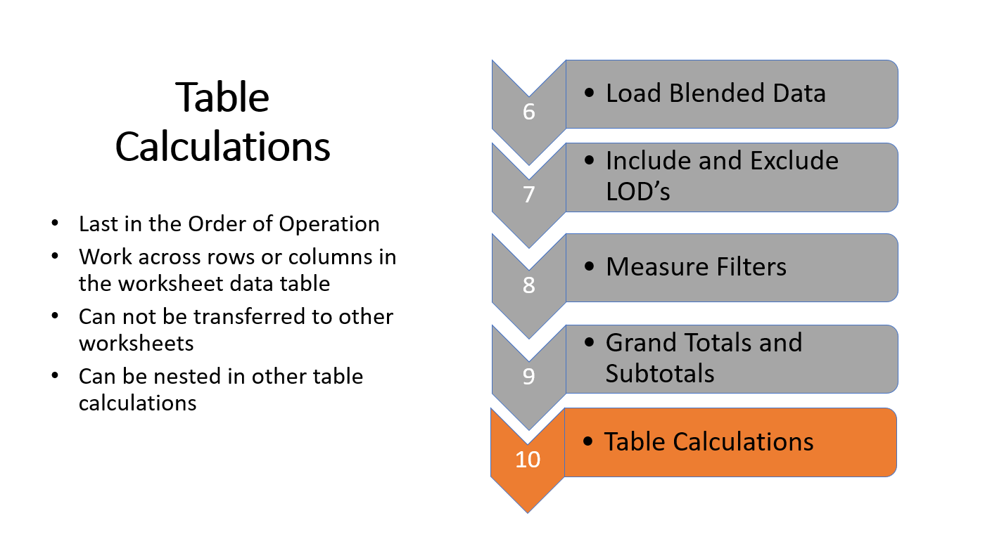
Table calculations are last in the order of operation and, in their basic form are easy to apply and understand – Most training programs introduce table calculations with a percent of total using a "Quick Table Calculation"
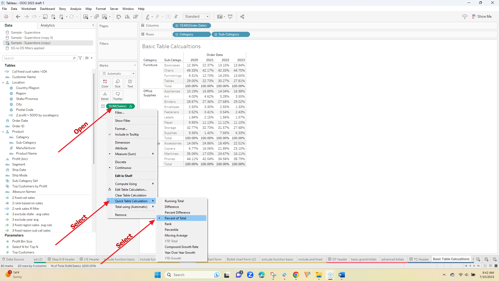
and then change the scope and direction using the Editor:
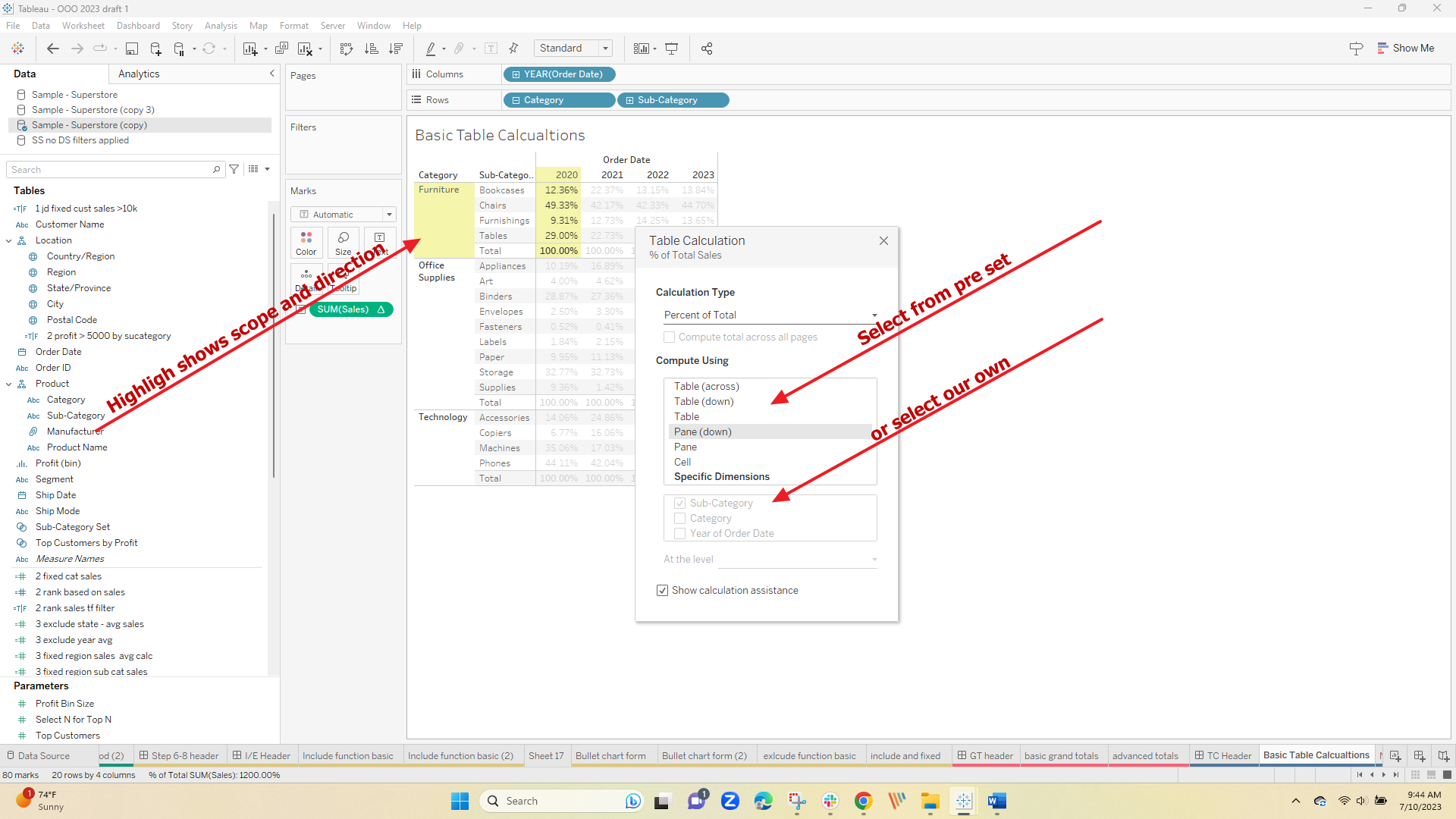
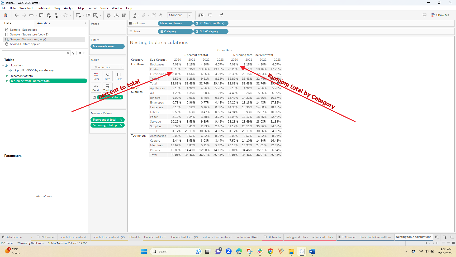
Easy enough, now let's move to a couple of more advanced calculations – the firsts nests 2 table calculations – Building upon the percent to total by adding a running total by category:
This is the basic percent to total calculation calculated down the table
SUM([Sales]) / TOTAL(SUM([Sales]))
That formula can be nested in another calculation that does a window sum on a running basis by category using this :
window_sum([5 percent of total ],FIRST(),0)
the optional start and stop say begin the total at the first record ( First()) and sub through the current (0).
and you can create your own
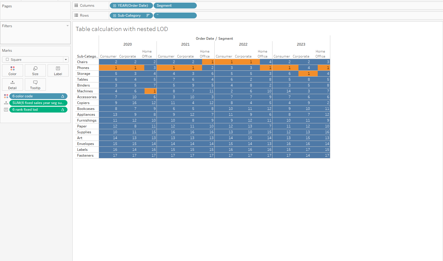
Early on you learned that you could not nest table calculations in LODs and that is true (you should understand why now) – but you can nest LODs in table calculations – In this use case we calculate the rank (a table calculation) of the segment, subcategory annual sales (an LOD):
First the LOD
{ FIXED year([Order Date]),[Segment],[Sub-Category]:sum([Sales])}
now the Rank table calculation – not the LOD needs to be aggregated with Sum():
RANK_UNIQUE(sum([6 fixed sales year seg sub cat]),'desc')
In text chart form with some formatting applied the result could look like this
I hope you better understand how you can leverage the Order of Operation when you need advanced calculations. The best way to learn now is to practice – make up your own examples or look for ways in your next example.
The workbook used here can be downloaded here Link to OOO Workbook
Enjoy
Jim