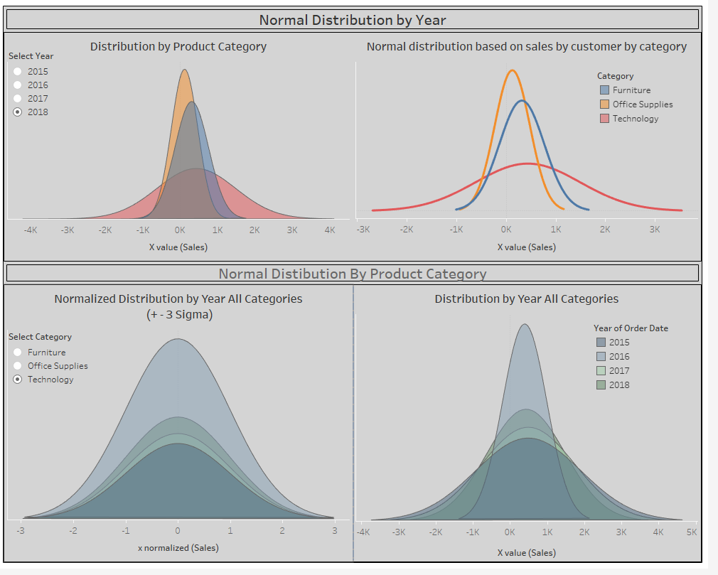
How to Create a Normal Distribution Chart

The approach here relies heavily on the concept of data densification develop and refined by Bora Beran, Joe Mako, Jonathan Drummey, Ken Flerlage, and others – Readers are encouraged to review their works on creating shapes and charts using the process.


This is a straightforward application of the normal distribution formula:
               

 
You may find more elegant approaches – when you do please let me know so we all can benefit

The data used here is the “Superstore” data set that comes with Tableau desktop –  while the data set is detailed down to the transaction level the examples here go to the Year/Category level – the concept can be adapted to any level in the Superstore data set or your own

Overview –

Tableau does not draw curved lines – so we simulate the familiar smooth bell curve of the normal distribution with a series of straight lines on an X-Y Cartesian coordinate grid.  The densification process is used to create intervals on the X-Axis (Sales in these examples).  As the number of intervals increases the plot becomes less angular. There is a parameter to adjust the number of intervals – somewhere between 50-100 intervals produces a reasonably smooth curve –play with it using your data to see what works for you

Step 1 Prepare the data for densification


Duplicate the data set by creating a union of the data with itself. Tableau will create a Dimension "Table Name" that can be used to distinguish the original data set from the duplicate – in the example the original data set is "Orders" and the duplicate in "Orders1"

 
Next, create a calculation to define the ends point needed for the X-values

Use the Path formula to create bins –

 
Step 2 – Create the X-values using the bins to pad the data – NOTE I used a +- 4 sigma range

First, determine the µ and σ values – the average and the standard deviation values in this example on Sales – but we want to be able to vary the results by year and by category

For that use, a LOD’s to create the needed combinations of year and category, and the widow function forces the calculation to be executed in each bin across the viz

Where  (index()-1) is the bin number (interval) on the x-axis

Step 3 – Solve the Normal Distribution formula for Y 

Table calculations are used to determine the Y value at each bin (x-value)
 
For clarity, there are 2 calculations 

The coefficient = (1/[σ*sqrt(2π])

                                 Coeff= 1/(sqrt(2*pi()*([sigma]^2)))

The Exponent =
                            Exponent = (-((([X value (Sales)])-[mu])^2)/((2*([sigma]^2)))  )
 
And then combined them in a single formula for Y (note Tableau does not have an "e" function but the EXP() will return the correct value)
                                                

 

Step 4 – Create the viz –

Place the X and Y values on columns and rows then add the Mu and Sigma values to the Detail tile

Then add Padded (the bins) to the viz and set the calculation across the bins (all places)

You can also make normalized distribution charts using the formula below

                x-normalized = ([mu]-[X value (Sales)])/[sigma]

and replace the x-value in any of the charts

 
Finally, I added a parameter and a filter to allow the user to change the number of standard deviations visible in the charts
               
 N-Std Dev Filter =  [x normalized (Sales)] >= -[enter number of standard deviations] and              [x normalized (Sales)]<=[enter number of standard deviations]
 

Place it on the filter shelf – it too is a table calculation set to use Padded – then set to True 

The workbook containing these examples and more can be found on my Tableau Public site at https://public.tableau.com/profile/jim.dehner#!/vizhome/Howtocreateanormaldistributionchart_v2018_3/summary

Jim